ECOC Model
This model can be trained with labeled genes in biological networks and then estimate label probabilities for any genes in the networks.
This description assumes that a label has been assigned to a set of known cooperating genes, and some other related labels have also been assigned to other genes in the training set. These labels can be fully customized from biological insights or generated computationally using gene set enrichment analysis (Please see this demo for more detail).
This learning and predicting process contain four essential components.
- propagate each label on a set of networks;
- aggregate the propagation results into an “error correction of code” matrix;
- learn the coding schema between labels and this ECOC matrix;
- predict labels for any genes in the ECOC matrix.
We’ll also explain the model’s hyperparameters and some additional implementation details. These implementations are for better data stratification, label probability estimation, and thresholding.
Multi-label space and network
Let’s start by defining the label space and networks. For \(q\) known labels and \(p\) genes, the gene labels can be expressed in both matrix and graph forms, such as the following toy example for two labels (red and blue).
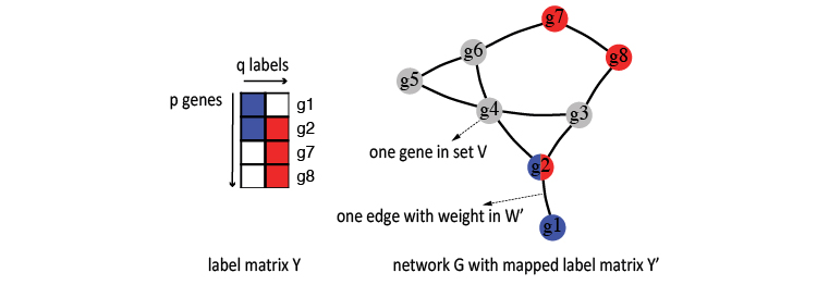
On the figure’s left side, this label space is expressed as a binary matrix \(Y\), where each \(y_{j}\) is a \(p\) element column vector filled with 1(colored) and 0(empty), denoting whether a gene is labeled or not.
\begin{equation} Y=\left(y_{1,},~y_{2}\text{, … ,}y_{j}\text{, … , }y_{q}\right) \end{equation}
On the right side of this figure, you can see the network (\(G\)) form with genes as nodes (\(V\)) and weighted edges(\(W'\)) for associations between them. Again, red and blue denote the labels.
\begin{equation} G=\left(V, W’\right) \end{equation}
Here, \(W'\) is the degree normalized weights, which is derived using the raw weights \(W\) and the network’s degree matrix \(D\).
\begin{equation} W’=D^{-1/2}WD^{-1/2} \end{equation}
Usually, in practice, we can only find a subset of these \(p\) genes in a network. We use another binary label matrix \(Y'\) to denote this overlapped portion, where \(y_{i\cdot}'=y_{i\cdot}\text{=1}\) (if gene \(i\) is found in this network).
Label propagation on a network
Following Vanunu et al., the algorithm starts by propagating the mapped label matrix \(Y'\) on the edge weight normalized networks, such as \(G\). Initially, all labeled genes in the network are assigned with value 1. These values are then propagated from the starting genes (such as \(g2\)) to their neighbor genes (such as \(g1,g3\) and \(g4\)).
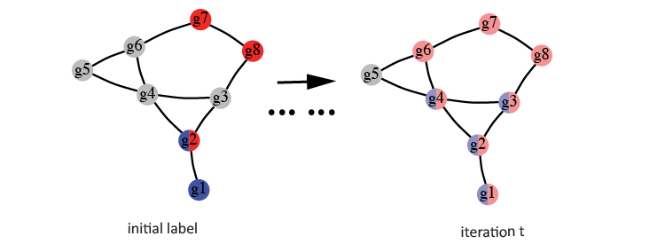
In this implementation, a parameter \(a\) controls the additionally infused label values from starting genes. Thus, this is also called a “Random Walk with Restart” process. Specifically, \(\left(1-a\right)\cdot y'_j\) additional label values are injected into the network at each iteration for each label \(j\). The following equation summarized this iteration process for updating a gene \(v\)’s label value for label \(j\).
\begin{equation} F_j\left(v\right)=a\left[\sum_{u\in Neighbor\left(v\right)}F_j\left(u\right)w’\left(v,u\right)\right]+\left(1-a\right)y_j’ \end{equation}
Here, \(w'(v,u)\) is from \(W'\) that denotes edge weight between gene \(u\) and \(v\). The algorithm continues this iterative process until the sum of label values changes drops below a threshold.
“Error correction of code” data matrix
Following the concept of “error correction of code”, the decoding error can be reduced in principle by repeatedly encoding each label \(n\) times from different biological perspectives. To obtain the encoded repetitive codewords as data matrix \(X\), this algorithm propagates each of the labels in \(Y\) on \(n\) diverse biological networks and stacks these values together.
 \begin{equation}
X=\left(x_{1},x_{2},…,x_{q\centerdot n}\right)
\end{equation}
\begin{equation}
X=\left(x_{1},x_{2},…,x_{q\centerdot n}\right)
\end{equation}
In practice, different iteration steps and starting label density generates these propagated values in different scales. To facilitate model training, they are normalized back to a \(\{0,m\}\) scale, where the maximum value \(m\) is defined as \(m=\sum y_{i}/p\), which is the proportion of genes with label \(i\). Also, a labeled gene is filled with this estimated maximum value of \(m\) in the data matrix \(X\), if it is missing in a network.
Coding schema
Using the propagated value matrix \(X\) and label matrix \(Y\), this algorithm learns a latent structure consisting of \(q\) labels and \(k\) label dependency terms. Following Zhang et al, this structure is defined as a codeword matrix \(Z\).
\begin{equation} Z= (Y,V^TY) \end{equation}

Here, the label matrix \(Y=(y_{1~},y_{2}\text{, ... , }y_{q} )\) represents the \(q\) labels. And the \(V^TY\) term denotes the most predictable label combination using feature matrix \(X\), so that the projection \(V\) mainly captures the conditional label dependency given \(X\) and its projection \(U\). The two projections are estimated with Canonical Correlation Analysis (CCA), which maximizes the correlations between the codewords \(Y\) and the data matrix \(X\).
Encoding and decoding
With the defined codeword matrix \(Z\) and encoded repetitive codes as data matrix \(X\), the algorithm can estimate the parameters for the latent coding structure to encode and decode. The figure below shows this process using 4 genes in the toy example.
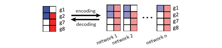
In encoding, a combination of linear and Gaussian regression models are used to encode codeword \(Z\) to the data matrix \(X\). The linear classifiers are for each of the \(q\) labels in \(Y\), and the gaussian regression models are for the \(k\) label dependency terms (\(V^TY\)). The following denotes the models for each row vector \(x^i\) in \(X\). In the toy example above, 4 row vectors for gene \(g1, g2, g7\) and \(g8\) are used to learn the latent structure of the 2 labels. The number of label dependency terms \(k\) is a hyperparameter to be estimated by cross validation.
\begin{equation} \phi_{j}\leftarrow linearClassifier\left(x^i,z_{j}\right),j\in1,…,q \end{equation}
\begin{equation} \psi_{j}\leftarrow GaussianRegression\left(x^i,z_{j}\right),j\in q+1,…,q+k \end{equation}
In decoding, this model decodes \(X\) to the codeword matrix \(Z\), where the first \(q\) columns are the probabilities for the \(q\) labels. The joint probability \(P\left(y\right)\) of labels for a row vector \(x^i\) can be summarized as the following.
\begin{equation} logP\left(y\right)=-logF+\lambda\sum_{j=1}^{q}\log\phi_{j}\left(y\right)+\sum_{d=1}^{k}\log\psi_{d}\left(y\right) \end{equation}
Here, \(F\) is the partition function and \(\lambda\) balances the two types of probabilities. In the second term, each of the linear classifier \(p_{j}\left(x\right)\) predicts a Bernoulli distribution for a label \(y_{j}\).
\begin{equation} \phi\left(y_{j}\right)=p_{j}\left(x\right)^{y_{j}}\left(1-p_{j}\left(x\right)\right)^{1-y_{j}},j=1,2,…,q \end{equation}
And the third term \(\sum_{d=1}^{k}\log\psi_{d}\left(y\right)\) is a set of \(k\) Gaussian regression models for the label dependencies.
\begin{equation} \psi_{d}\left(y\right)\sim exp^{-\left(v_{d}^{T}y-m_{d}\left(x\right)\right)^{2}/2\sigma_{d}^{2},~},d=1,2,…,k \end{equation}
Here, \(m_{d}\left(x\right)\) is the regression model and \(\sigma_{d}^{2}\) is estimated by cross validation in training. A mean-field approximation is used for estimating \(P\left(y\right)\) in this implementation.
\begin{equation} Q\left(y\right)=\prod_{j=1}^{q}Q_{j}\left(y_{j}\right) \end{equation}
It is fully factorized and each \(Q_{j}\left(y_{j}\right)\) in \(Q\left(y\right)\) is a Bernoulli distribution on the label \(y_{j}\). The best approximation \(Q\left(y\right)\) is obtained by minimizing the KL divergence between \(Q\left(y\right)\) and \(P\left(y\right)\).
\begin{equation} KL\left(Q(y)\vert P(y)\right) \end{equation}
Second-order iterative stratification
It is not trivial for dividing the training data to subsets in the context of gene function prediction algorithms, especially in a multi-label setting. Many of these labels are much less than the total number of genes in a species. With these small positive label ratio, random subsets can not preserve the same label dependencies as in the whole training data. This implementation uses a second-order iterative stratification heuristic (Szymański and Kajdanowicz, 2017; Sechidis et al., 2011) to distribute the positive labels while maintaining the label ratios close to the entire training set.
Probability calibration
This implementation automatically estimates \(q\) thresholds for all labels’ probabilities based on the harmonic mean of precision and recall (Fan and Lin, 2007; Zou et al.,2016). However, the raw probabilities estimated from this multi-label model is often skewed. As a result, a little change in the probability threshold can dramatically change the prediction outcome. Thus, a Platt’s scaling heuristic (Lin et al.,2007; Platt, 1999) is integrated into this model to calibrate the probabilities for robust threshold estimations in practice. In addition, as some genes’ labels are still unknown, it is easy to come across false negatives in training data, which confuses this logistic regression based calibration process. So, the calibration is further modified to reduce the influence of false negatives (Rüping, 2006). This modification may remove a part of top predictions in training for a better estimation for calibration parameters, determined by the mean squared error in regression.
Hyperparameters
Two hyperparameters are estimated in training, which are \(k\) dependency terms in the coding schema and \(\lambda\) that balance the linear classifier and the Gaussian regression models for decoding. The sub-command ecoc tune will automatically estimate them in training. They can also be specified directly in sub-command ecoc pred.
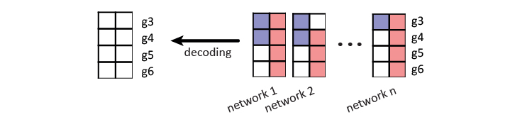
Gene label prediction
The final step is to decode \(X\) to a predicted label matrix \(Y^h\), using the learned \(q\) linear models and \(k\) label dependency terms. In the mentioned toy example throughout this page, the labels and repetitive codes for gene \(g1, g2, g7\), and \(g8\) are used for training the model. And the repetitive code for gene \(g3, g4, g5\), and \(g6\) are decoded back to label probabilities. These are the label predictions for these four genes.
References
- Fan, R.-E., and Lin, C.-J. (2007). A study on threshold selection for multi-label classification. Department of Computer Science, National Taiwan University.
- Lin, H.-T., Lin, C.-J., and Weng, R. C. (2007). A note on Platt’s probabilistic outputs for support vector machines. Machine Learning.
- Platt, J. C. (1999). Probabilistic Outputs for Support Vector Machines and Comparisons to Regularized Likelihood Methods. In ADVANCES IN LARGE MARGIN CLASSIFIERS.
- Rüping, S. (2006). Robust Probabilistic Calibration. In Machine Learning: ECML 2006.
- Sechidis, K., Tsoumakas, G., and Vlahavas, I. (2011). On the stratification of multi-label data. Machine Learning and Knowledge Discovery in Databases.
- Szymański, P., and Kajdanowicz, T. (2017). A Network Perspective on Stratification of Multi-Label Data. In Proceedings of the First International Workshop on Learning with Imbalanced Domains: Theory and Applications.
- Vanunu, O., Magger, O., Ruppin, E., Shlomi, T., and Sharan, R. (2010). Associating genes and protein complexes with disease via network propagation. PLoS computational biology.
- Zhang, Y. and Schneider, J. (2011). Multi-Label Output Codes using Canonical Correlation Analysis. In Proceedings of the Fourteenth International Conference on Artificial Intelligence and Statistics.
- Zou, Q., Xie, S., Lin, Z., Wu, M., and Ju, Y. (2016). Finding the Best Classification Threshold in Imbalanced Classification. Big Data Research.